On Wednesday March 6 we’ll kick off our Crime Data Analysis project, and before then, it may be worth asking “Why are a bunch of amateurs attempting what the police should be doing? " The answer is that police departments analyze crime to catch criminals, and the Data Library analyzes crime to help residents understand their own communities. We data geeks aren’t very good at catching criminals, so we’re happy to leave that task to the pros. Our project will cover only two small aspects of the field of Crime Analysis. We’ll be doing strategic analysis, looking at long term trends, and descriptive administrative analysis, which is creating summary reports for community leaders. So, some of the activities that we’ll tackle as part of this project are:
Fight Crime with Data
Citizens of any skill level are invited to help us analyze crime in San Diego neighborhoods. Use your knowledge of the community or technical skill to create maps, discover anomalies, and better understand the causes and solutions to crime in San Diego. Come to the Kickoff meeting by signing up at Meetup.com Crime is always a top issue for any community, but San Diego residents, town councils and community planning groups seldom see neighborhood analysis of where crime occur, and less frequently get analysis of how crime relates to factors such as street lighting, traffic, housing, or alcohol. In this project we will collect data from the city, state and private organizations to create a range of maps and statistics that explain where crime is occurring and what factors are involved in increases or decreases in crime. This project needs your help,regardless of your skills or skill level. You can participate as a non technical community activist, Excel jockey, GIS expert, beginning programmer or experienced statistician. Want to know more?
Property vs Violent Crime
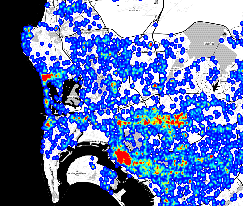
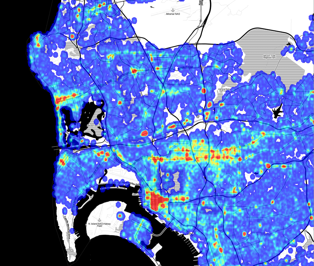
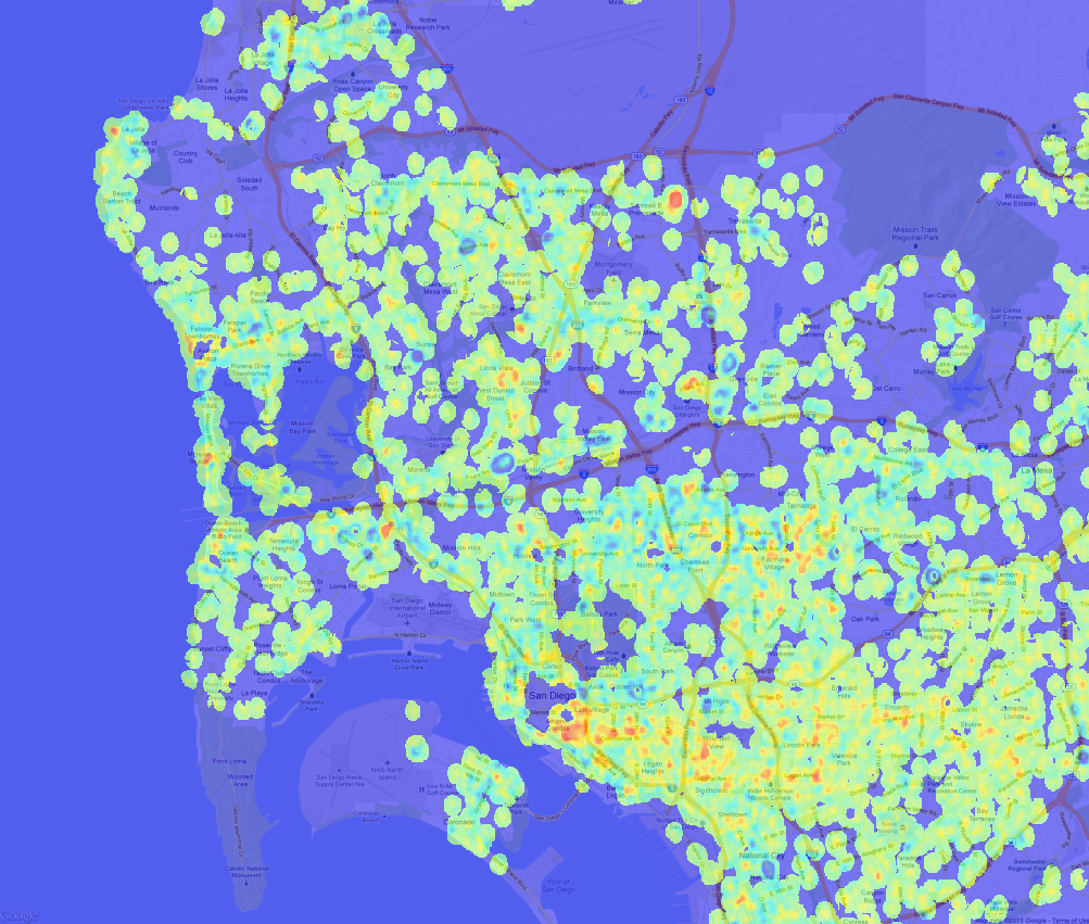
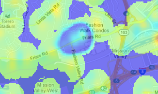
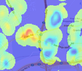
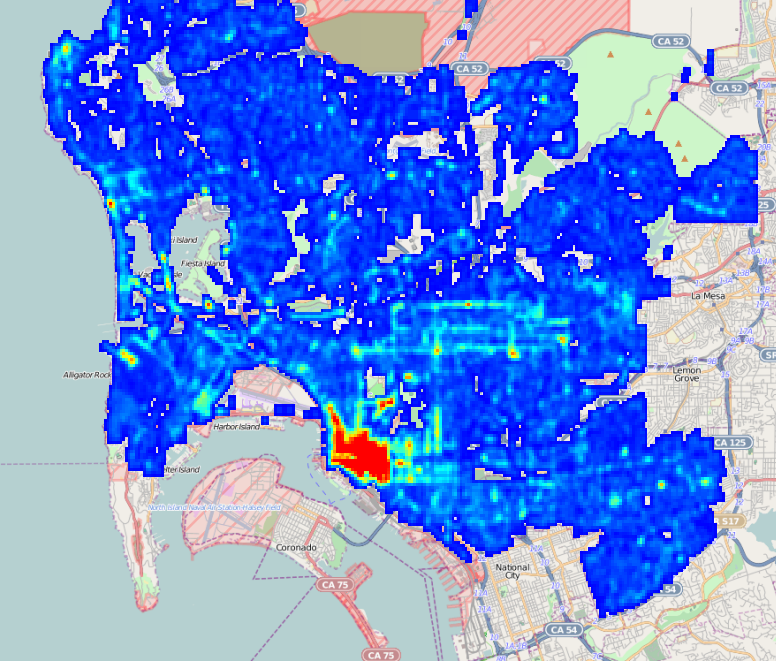
As part of our upcoming Crime Mapping project, we’ve started producing maps of San Diego area cime incidents, and have made a few interesting discoveries that we’d like to share. While these aren’t ground-breaking insights, the results do confirm intuition and offer some small surprises. A few months ago we received and processed the SpotCrime.com free database, a database of crime incidents from across the country for the years 2007 to 2011. This data was scraped from many different police department websites, although the San Diego data was all scraped from ARJIS ( part of SanDAG ) before SANDAG changed the map software, eliminating the possibility of free acess. This database is a wonderful resource, and even though the data does not have an official pedigree, there are enough datapoints to do some useful work. SpotCrime is providing an incredible benefit by offering this data. Thanks! Our first stage of analysis involves creating heatmaps from the incidents. To create these maps, we quantized the incidents into bins 1/5000 of a degree square, about 19m. Since the records are typically reported with a “hundred block address” – “1300 Wilbur Ave” instead of “1324 Wilbur Ave” – we added a bit of randomness to the points. While this isn’t exactly correct, as it randomly moves the incident by up to 100m, it does space the points out in a more natural way. Then, for each incident, we spread out the crime point ( with a 2-D Gaussian, fwhm = 57m) to smooth out the image. The spreading also simulates both the extended “influence” of a crime, and the fact that a crime at one point means it is more probable that a crime will occur at nearby points. Violent crimes are separated from from the property crimes with a separate map for each. Here is the violent crime map: ( Click to Enlarge) Violent Crime Incidents, 2007 - 2011. Data from SpotCrime.com The red spots are the areas of the highest number of crimes, and almost all of them are entertainment districts. Violent crime tends to occur at night, where there are a lot of people, and where people are drinking, and an entertainment district has all three conditions. Here is the map of the property crime incidents. This has more complete coverage because there are a lot more property crime incidents than violent crime incidents. Property Crime Incidents, 2007 to 2011. Data from SportCrime.com There are a lot of similarities in where the crimes occur, but the property crimes are more diffuse, and there are many small-scale differences. To find the differences between the two, we can subtract the two maps. In this image, blue indicates areas where property crimes dominate, green is neutral, and red is an area where violent crimes dominate: Violent crime density minus property crime density. Note that in this map, green does not mean “good,” it means that the difference in the density of violent crime and property crime is nearly equal. The green areas can have very high violent crime rates; being green just means they also have high property crime rates. This map gets really interesting when you zoom in to look at specific spots. Closer examination doesn’t reveal a lot of new discoveries, but it does confirm intuition about where we should find property and violent crimes. ![]() | This high-property crime area is Fashion Valley Mall. It seems sensible that the mall would be a target for theft, but the upscale shoppers don’t often get into altercations. Mission Valley mall has a similar emphasis on property crimes. |
|---|---|
![]() | Qualcomm stadium, in red, is a hot spot for rowdy sports crowds, but the apartments along the golf course, while actually having a higher than average violent crime rate, see relatively more property crime. |
| (There is an interesting error in the difference map. The values for each map are scaled so that the range of ±4σ in the original output maps to (0,1] in the final output, so high outliers all have the value of exactly 1. This means that for an area with both high property and violent crime, the difference is exactly 0, which is the no data value. This is why Garnet street in Pacific Beach and the Gaslamp district have areas of no data in the difference map. ) A map like this has a lot of interesting stories to tell, even though the analysis is not very rigorous. We started with data that we can’t vouch for, added randomness, created a map with a lot of arbitrary choices, and ended up with useful insights. The entire process emphasizes that even when data and analysis are not of sufficient quality to make statistical inferences, we can still extract useful knowledge. |
Crime And Street Lamps
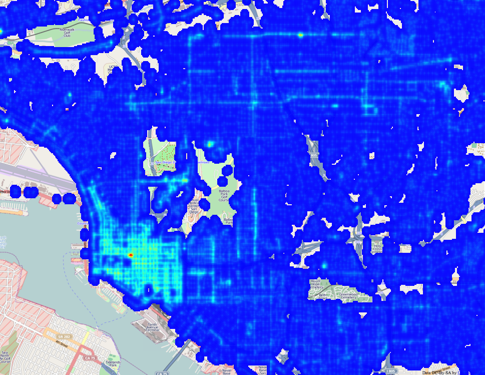
In preparing to formally launch the San Diego Regional Data Library, we’ve been spending a lot of time talking to nonprofits, community planing groups, city staff and city council members about their data needs. The staff for District 9 mentioned that Council member Marti Emerald is interested in infrastructure issues, particularly how crime is related to infrastructure deficits. Her staff specifically mentioned street lamps. Fortunately, we have a fantastic resource in SanGIS, and they have published a shapefile with the locations of San Diego Street Lamps. So, we went to work extracting and processing street lamp data. Based on this data, we’re creating density maps of street lights, which we will correlate with crime incidents. The map shown here is one of the example maps we’ve produced, to experiment with how best to represent the data. For this map, I wrote a Data Bundle that converted the Shapefile of street lights provided by SanGIS into a Sqlite file, which was then loaded into an image. ( You can get the code for my bundle on GitHub. ) The processing code bins the location of the street lights to 1/4000 of a degree, about 18 meters at out latitude, then for each street lamp, adds a matrix onto the output image. The matrix spreads out the point, a bit like the light from the lamp would spread out. Here is a high resolution view of the output, showing Uptown, Downtown , the Park and Golden Hill. ( Click to expand )
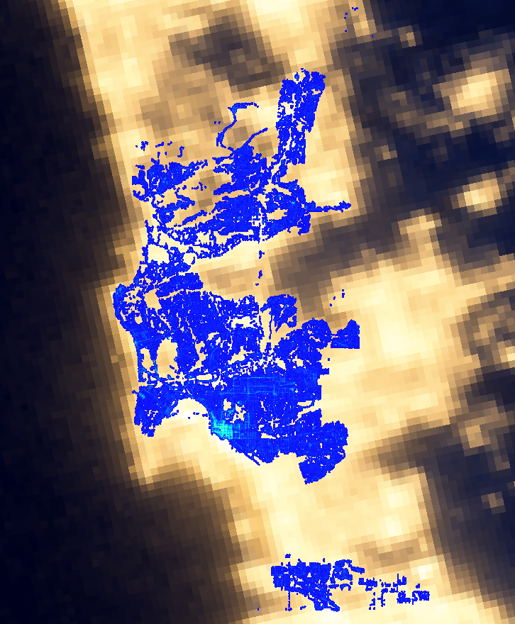
This is, of course, a synthetic view of light in San Diego, but NASA has generated the real view, by photographing the earth at night. Here is our map laid over NASA’s image:
Our data covers only San Diego, so there are many areas that are lit where we don’t have street lamp records, and it also appears that from space, light spreads much more than we estimate with our spreading matrix. Regardless, the maps show a good correspondence. This is a simplistic analysis, since it doesn’t consider the different types of lamps, their power, or the occlusion of buildings, but it does illustrate how to make and present a density map. This is the first step in our crime analysis project; the next steps will study how the locations of street lamps relate to the locations of crime. For the full project, we will have to consider that the correlation between crime and street lights isn’t only one way. There may be more crime in dark areas, but the city may also put more lights in high crime areas, breaking a simple correlation. So, we will probably focus on finding areas that are both dark and have high crime. If you like this sort of analysis, please join our Meetup group or connect though Facebook, Twitter or email to get the announcement for the start of our crime analysis project. We’d love to have your help!
San Diego Civic Engagement
The Corporation for National and Community Service is a federal agency that encourages US citizens to volunteer, particularly for federal programs like AmeriCorps. They also have an excellent data site that provides statistics on civic engagement. We used their data extraction tool to pull a few datasets, which are posted on the Library’s data repository. Here is a bar chart of the percentage of the population of large US cities which, in the previous 12 months, volunteered for a formal organization. The chart shows the averages for the years 2004 to 2011, including the standard deviation from year to year for a single city as an error bar. The numbers on the right indicate rank.